L1 loss, abs L1 loss, and L2 loss

5 min readMay 2, 2020

We are commonly using L2 loss in deep learning. My question is why not use L1 loss? Here, I’d like to do an experiment to explain.

Experiment setup

we are going to estimate

wx = y

where we only have one parameter which is w and in order to make the problem even simple, we’d like also fix the value of x by picking up a value of 2 for x.

So what we are going to estimate is

2*w = y

For the regular wx+b=y estimation, please check this code.

we set the unknow w as 1 and we are going to estimate this w.

Code

prepare the data

# simulate the l1 loss and l2 loss
# simulate w*x = y where x is a fixed number 2
# It means we are going to simulate 2*w = y
# a noise item will be added which is z. 
# 2*w + z = y
# if z is 0, then there is no noise, 
# else some gaussian noise will be added
import numpy as np
import random
import matplotlib.pyplot as plt
# number of samples
N = 20
INIT_w = 20
# our target w is 1.0add_noise = False
x = 2*np.ones((N,))
if add_noise:
    z = np.random.normal(0, 0.05, N)
    y = 1.0*x + z
else:
    y = 1.0*x

Define the loss

def loss(y_hat, y, loss='L1'):
    if loss=='L1':
        print('L1 loss')
        return  np.sum(y_hat - y)
    elif loss == 'L2':
        print('L2 loss')
        return np.sum(np.square(y_hat-y))

Train the model using a gradient descent algorithm

epoches = 20
batch_size = 2
batch_start_idx = list(range(0, N, batch_size))l1_losses, l2_losses = [], []
w_l1_loss, w_l2_loss = [], []
# set learning rate as 1.0
lr = 0.01for loss_type in ['L1', 'L2']:
    w = INIT_w 
    for epoch in range(epoches):
        for batch_i in batch_start_idx:
            this_x, this_y = x[batch_i:batch_i+batch_size], y[batch_i:batch_i+batch_size]
            y_hat = w*this_x
            L = loss(y_hat, this_y, loss_type)
            if loss_type == 'L1':
                l1_losses.append(L)
                print(f"{loss_type}, {L}")
                # L = y_hat -y , dL/dy_hat = 1
                # dy_hat/dw = x
                # dL/dw = 1*x
                gradient = np.sum(x)
                print(gradient)
                w -= lr*gradient
                w_l1_loss.append(w)
            elif loss_type == 'L2':
                l2_losses.append(L)
                print(f"{loss_type}, {L}")
                # L = (y_hat -y)**2 , dL/dy_hat = 2(y_hat - y)
                # dy_hat/dw = x
                # dL/dw = 2(y_hat-y)*x
                gradient = np.sum(2*(y_hat-this_y)*this_x)
                w -= lr*gradient
                w_l2_loss.append(w)

Visualization of the algorithm

plt.plot(range(len(l1_losses)), l1_losses, c = 'r', label='L1 loss')
plt.plot(range(len(l2_losses)), l2_losses, c = 'g', label='L2 loss')
plt.xlabel('step')
plt.ylabel('loss')
if add_noise:
    plt.title('initialize w:'+str(INIT_w)+' with noise')
else:
    plt.title('initialize w:'+str(INIT_w)+' without noise')
plt.legend(loc='best')
if add_noise:
    plt.savefig('loss_l1_l2_with_noise.png')
else:
    plt.savefig('loss_l1_l2_without_noise.png')
plt.show()
plt.close()
plt.plot(range(len(w_l1_loss)), w_l1_loss, c = 'r', label='L1 loss')
plt.plot(range(len(w_l2_loss)), w_l2_loss, c = 'g', label='L2 loss')
plt.xlabel('step')
plt.ylabel('estimate w (target is 1)')
if add_noise:
    plt.title('initialize w:'+str(INIT_w)+' with noise')
else:
    plt.title('initialize w:'+str(INIT_w)+' without noise')
plt.legend(loc='best')
if add_noise:
    plt.savefig('w_l1_l2_with_noise.png')
else:
    plt.savefig('w_l1_l2_without_noise.png')
plt.show()

The full code

Full code can get from here:

liketheflower/linear_gradient_descent

Contribute to liketheflower/linear_gradient_descent development by creating an account on GitHub.

github.com

Visualization results

L1 loss can be negative and l2 loss is approaching 0

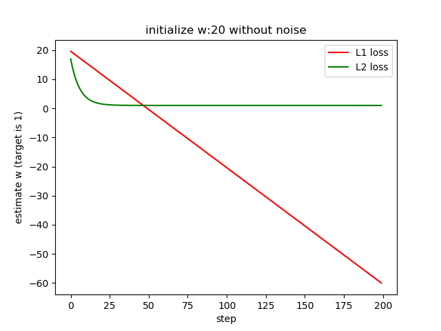
From the second plot, we can see by using L1 loss, the estimation fails as the gradient descent algorithm will push the loss function go to a smaller value. So by using L1 loss, it fails. If we keep on training, the w will go to -inf.

What if we change the L1 loss to abs L1 loss?

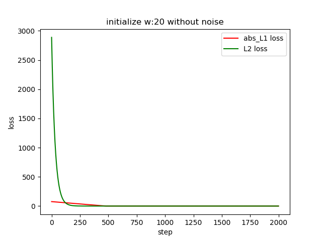
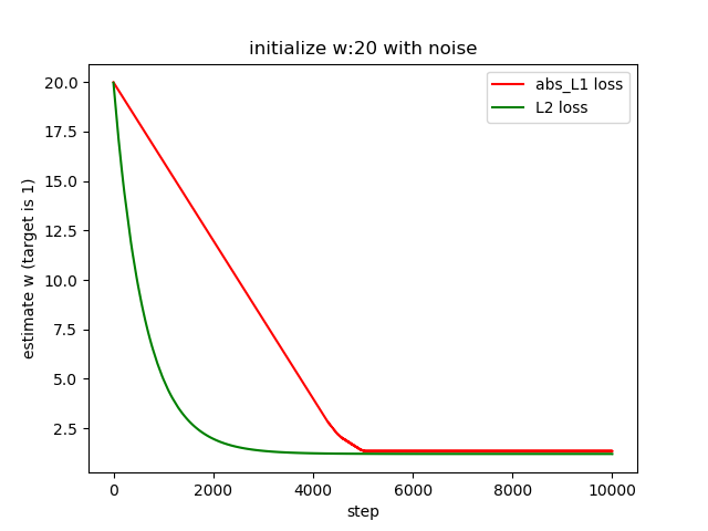
Yes, it works. However, the L2 loss converges much faster as L2 loss has a larger gradient when far away from the zero gradients. While the L1 loss is kind of stable.

What about adding some noise

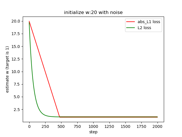
Gaussian noise is added with mean as 0 and standard deviation as sigma.

When sigma is small which is 0.05, we have

When sigma is large say sigma = 5

Loss is not stable if we use L2 loss as L2 loss is more sensitive to noise

The estimation based on L2 loss is better.

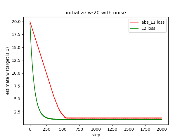
The estimation of L2 is better than based on abs L1 loss. We believe it is because the L2 gradient will be reduced if it is close to the global minimum. However, for the abs L1 the magnitude of the gradient keeps the same.

How to address this issue?

Approach 1: using a smaller learning rate

current learning rate = 0.001

change it to 0.0001

We need more iterations in this case and the results of abs L1 loss is better than before.

Also we can use an exponential decay learning rate.

we reset the learning rate to 0.01 and decay = 1/2000

lr = init_lr*(1. / (1. + decay * iterations))

When the learning rate is small, the updating process will be dominated by the gradient. The gradient will have fluctuations with the noise. This explains why the update of w has fluctuated.

Code related to abs l1 loss

Code for this part is in the same repo as the previous one and the code name is:abs_l1_l2_loss.py

Thanks for reading.